One-factor-at-a-time simulations
The module pnptransport.parameter_span provides functions to multiple input files necessary to simulate the effect of the variation of a specific parameter.
The following scripts provides an example of the usage:
1 2 3 4 5 6 7 8 9 10 11 12 13 14 15 16 17 18 19 20 21 22 23 24 25 26 27 28 29 30 31 32 33 34 35 36 37 38 39 40 41 42 43 44 45 | """
This program will create all the necessary input files to run pnp transport simulations with 'one factor at a time'
variations.
The variations on the relevant parameters are described in pidsim.parameter_span.one_factor_at_a_time documentation.
These variations are submitted through a csv data file.
The rest of the parameters are assumed to be constant over all the simulations.
Besides the input files, the code will generate a database as a csv file with all the simulations to be run and the
parameters used for each simulation.
@author: <erickrmartinez@gmail.com>
"""
import numpy as np
import pidsim.parameter_span as pspan
# The path to the csv file with the conditions of the different variations
csv_file = r'G:\My Drive\Research\PVRD1\Manuscripts\Device_Simulations_draft\simulations\one_factor_at_a_time_lower_20201028_h=1E-12.csv'
# Simulation time in h
simulation_time_h = 96.
# Temperature in °C
temperature_c = 85
# Relative permittivity of SiNx
er = 7.0
# Thickness of the SiNx um
thickness_sin = 75E-3
# Modeled thickness of Si um
thickness_si = 1.0
# Number of time steps
t_steps = 1440
# Number of elements in the sin layer
x_points_sin = 100
# number of elements in the Si layer
x_points_si = 100
# Background concentration in cm^-3
cb = 1E-20
if __name__ == '__main__':
pspan.one_factor_at_a_time(
csv_file=csv_file, simulation_time=simulation_time_h*3600, temperature_c=temperature_c, er=er,
thickness_sin=thickness_sin, thickness_si=thickness_si, t_steps=t_steps, x_points_sin=x_points_sin,
x_points_si=x_points_si, base_concentration=cb
)
|
The script will use the csv file defined in csv_file which has the following form
| Parameter | base | span |
|---|---|---|
| sigma_s | 1.00E+10 | 1E10,1E11,1E12,1E13,1E14 |
| zeta | 1.00E-04 | 1E-8, 1E-7, 1E-6, 1E-5,1E-4 |
| DSF | 1.00E-14 | 1E-14,1E-15,1E-16 |
| E | 1.00E+04 | 1E1,1E2,1E3,1E4,1E5,1E6 |
| m | 1.00E+00 | 1 |
| h | 1.00E-12 | 1E-12,1E-10,1E-8 |
| recovery time | 43200 | 43200 |
| recovery electric field | -1.00E+04 | -1.00E+04 |
sigma_s corresponds to the surface concentration at the source \(S\) in cm-2 , zeta corresponds to the rate of ingress from the source \(k\) in s-1 , DSF is the diffusivity of Na in the stacking fault \(D_{\mathrm{SF}}\) in cm2/s, E is the electric field in SiNxgiven in V/cm, h and m are the surface mass transfer coefficient (cm/s) and segregation coefficient at the SiNx/Si interface, respectively. The recovery time is indicated in seconds and corresponds to time added to the simulation where the system is either (1) allowed to relax by removing the electric stress or, (2) stressed under the PID stress in reverse polarity. The value of the recovery electric field is indicated in the last row of the table.
The column base corresponds to the base case to compare the rest of the simulations. The span column indicates all the variations from the base case for the respective parameter in the row, while keeping the rest of the parameters constant.
After running the code, the following file structure will be created
which will generate a folder structure like this.
base_folder
|---one_factor_at_a_time.csv
|---input
|   |---constant_source_flux_96_85C_1E+10pcm2_z1E-04ps_DSF1E-14_1E+01Vcm_h1E-12_m1E+00_rt12h_rv-1E+01Vcm.ini
|   |---constant_source_flux_96_85C_1E+10pcm2_z1E-04ps_DSF1E-14_1E+02Vcm_h1E-12_m1E+00_rt12h_rv-1E+02Vcm.ini
|   |--- ...
|   |---ofat_db.csv
|   |---batch_YYYYMMDD.sh
With \(n\) .ini files corresponding to all of the variations. The naming convention for the .ini files is constant_source_flux_ + PID stress time in hours + _ + \(T\) in °C + C_ + \(S\) in cm-2+ pcm2_z + \(k\) in s-1 + ps_DSF + \(D_{\mathrm{SF}}\) in cm2/s + _ + \(E\) in V/cm + _h + \(h\) in cm/s + _m + \(m\) + _rt + recovery time in hours + h_rv + recovery voltage (at the SiNx) in V/cm.
Additionally, the scripts create a batch script batch_YYYYMMDD.sh that needs to be run in the location where simulate_fs.py can be reached. This will send all the simulations as separate python jobs to the OS.
Lastly, the script generates a ofat_db.csv table containing the list of all simulations with all the parameters used in each case:
| config file | sigma_s (cm^-2) | zeta (1/s) | D_SF (cm^2/s) | E (V/cm) | h (cm/s) | m | time (s) | temp (C) | bias (V) | recovery time (s) | recovery E (V/cm) | recovery bias (V) | thickness sin (um) | thickness si (um) | er | cb (cm^-3) | t_steps | x_points sin | x_points si |
|---|---|---|---|---|---|---|---|---|---|---|---|---|---|---|---|---|---|---|---|
| constant_source_flux_96_85C_1E+10pcm2_z1E-04ps_DSF1E-14_1E+04Vcm_h1E-12_m1E+00_rt12h_rv-1E+04Vcm.ini | 10000000000 | 0.0001 | 1.00E-14 | 10000 | 1.00E-12 | 1 | 345600 | 85 | 0.075 | 43200 | -10000 | -0.075 | 0.075 | 1 | 7 | 1.00E-20 | 720 | 100 | 100 |
| constant_source_flux_96_85C_1E+11pcm2_z1E-04ps_DSF1E-14_1E+04Vcm_h1E-12_m1E+00_rt12h_rv-1E+04Vcm.ini | 1E+11 | 0.0001 | 1.00E-14 | 10000 | 1.00E-12 | 1 | 345600 | 85 | 0.075 | 43200 | -10000 | -0.075 | 0.075 | 1 | 7 | 1.00E-20 | 720 | 100 | 100 |
| constant_source_flux_96_85C_1E+12pcm2_z1E-04ps_DSF1E-14_1E+04Vcm_h1E-12_m1E+00_rt12h_rv-1E+04Vcm.ini | 1E+12 | 0.0001 | 1.00E-14 | 10000 | 1.00E-12 | 1 | 345600 | 85 | 0.075 | 43200 | -10000 | -0.075 | 0.075 | 1 | 7 | 1.00E-20 | 720 | 100 | 100 |
| constant_source_flux_96_85C_1E+13pcm2_z1E-04ps_DSF1E-14_1E+04Vcm_h1E-12_m1E+00_rt12h_rv-1E+04Vcm.ini | 1E+13 | 0.0001 | 1.00E-14 | 10000 | 1.00E-12 | 1 | 345600 | 85 | 0.075 | 43200 | -10000 | -0.075 | 0.075 | 1 | 7 | 1.00E-20 | 720 | 100 | 100 |
| constant_source_flux_96_85C_1E+14pcm2_z1E-04ps_DSF1E-14_1E+04Vcm_h1E-12_m1E+00_rt12h_rv-1E+04Vcm.ini | 1E+14 | 0.0001 | 1.00E-14 | 10000 | 1.00E-12 | 1 | 345600 | 85 | 0.075 | 43200 | -10000 | -0.075 | 0.075 | 1 | 7 | 1.00E-20 | 720 | 100 | 100 |
| constant_source_flux_96_85C_1E+10pcm2_z1E-08ps_DSF1E-14_1E+04Vcm_h1E-12_m1E+00_rt12h_rv-1E+04Vcm.ini | 10000000000 | 1.00E-08 | 1.00E-14 | 10000 | 1.00E-12 | 1 | 345600 | 85 | 0.075 | 43200 | -10000 | -0.075 | 0.075 | 1 | 7 | 1.00E-20 | 720 | 100 | 100 |
| constant_source_flux_96_85C_1E+10pcm2_z1E-07ps_DSF1E-14_1E+04Vcm_h1E-12_m1E+00_rt12h_rv-1E+04Vcm.ini | 10000000000 | 1.00E-07 | 1.00E-14 | 10000 | 1.00E-12 | 1 | 345600 | 85 | 0.075 | 43200 | -10000 | -0.075 | 0.075 | 1 | 7 | 1.00E-20 | 720 | 100 | 100 |
| constant_source_flux_96_85C_1E+10pcm2_z1E-06ps_DSF1E-14_1E+04Vcm_h1E-12_m1E+00_rt12h_rv-1E+04Vcm.ini | 10000000000 | 1.00E-06 | 1.00E-14 | 10000 | 1.00E-12 | 1 | 345600 | 85 | 0.075 | 43200 | -10000 | -0.075 | 0.075 | 1 | 7 | 1.00E-20 | 720 | 100 | 100 |
| constant_source_flux_96_85C_1E+10pcm2_z1E-05ps_DSF1E-14_1E+04Vcm_h1E-12_m1E+00_rt12h_rv-1E+04Vcm.ini | 10000000000 | 1.00E-05 | 1.00E-14 | 10000 | 1.00E-12 | 1 | 345600 | 85 | 0.075 | 43200 | -10000 | -0.075 | 0.075 | 1 | 7 | 1.00E-20 | 720 | 100 | 100 |
| constant_source_flux_96_85C_1E+10pcm2_z1E-04ps_DSF1E-15_1E+04Vcm_h1E-12_m1E+00_rt12h_rv-1E+04Vcm.ini | 10000000000 | 0.0001 | 1.00E-15 | 10000 | 1.00E-12 | 1 | 345600 | 85 | 0.075 | 43200 | -10000 | -0.075 | 0.075 | 1 | 7 | 1.00E-20 | 720 | 100 | 100 |
| constant_source_flux_96_85C_1E+10pcm2_z1E-04ps_DSF1E-16_1E+04Vcm_h1E-12_m1E+00_rt12h_rv-1E+04Vcm.ini | 10000000000 | 0.0001 | 1.00E-16 | 10000 | 1.00E-12 | 1 | 345600 | 85 | 0.075 | 43200 | -10000 | -0.075 | 0.075 | 1 | 7 | 1.00E-20 | 720 | 100 | 100 |
| constant_source_flux_96_85C_1E+10pcm2_z1E-04ps_DSF1E-14_1E+01Vcm_h1E-12_m1E+00_rt12h_rv-1E+01Vcm.ini | 10000000000 | 0.0001 | 1.00E-14 | 10 | 1.00E-12 | 1 | 345600 | 85 | 7.50E-05 | 43200 | -10 | -7.50E-05 | 0.075 | 1 | 7 | 1.00E-20 | 720 | 100 | 100 |
| constant_source_flux_96_85C_1E+10pcm2_z1E-04ps_DSF1E-14_1E+02Vcm_h1E-12_m1E+00_rt12h_rv-1E+02Vcm.ini | 10000000000 | 0.0001 | 1.00E-14 | 100 | 1.00E-12 | 1 | 345600 | 85 | 0.00075 | 43200 | -100 | -0.00075 | 0.075 | 1 | 7 | 1.00E-20 | 720 | 100 | 100 |
| constant_source_flux_96_85C_1E+10pcm2_z1E-04ps_DSF1E-14_1E+03Vcm_h1E-12_m1E+00_rt12h_rv-1E+03Vcm.ini | 10000000000 | 0.0001 | 1.00E-14 | 1000 | 1.00E-12 | 1 | 345600 | 85 | 0.0075 | 43200 | -1000 | -0.0075 | 0.075 | 1 | 7 | 1.00E-20 | 720 | 100 | 100 |
| constant_source_flux_96_85C_1E+10pcm2_z1E-04ps_DSF1E-14_1E+05Vcm_h1E-12_m1E+00_rt12h_rv-1E+05Vcm.ini | 10000000000 | 0.0001 | 1.00E-14 | 100000 | 1.00E-12 | 1 | 345600 | 85 | 0.75 | 43200 | -100000 | -0.75 | 0.075 | 1 | 7 | 1.00E-20 | 720 | 100 | 100 |
| constant_source_flux_96_85C_1E+10pcm2_z1E-04ps_DSF1E-14_1E+06Vcm_h1E-12_m1E+00_rt12h_rv-1E+06Vcm.ini | 10000000000 | 0.0001 | 1.00E-14 | 1000000 | 1.00E-12 | 1 | 345600 | 85 | 7.5 | 43200 | -1000000 | -7.5 | 0.075 | 1 | 7 | 1.00E-20 | 720 | 100 | 100 |
| constant_source_flux_96_85C_1E+10pcm2_z1E-04ps_DSF1E-14_1E+04Vcm_h1E-10_m1E+00_rt12h_rv-1E+04Vcm.ini | 10000000000 | 0.0001 | 1.00E-14 | 10000 | 1.00E-10 | 1 | 345600 | 85 | 0.075 | 43200 | -10000 | -0.075 | 0.075 | 1 | 7 | 1.00E-20 | 720 | 100 | 100 |
| constant_source_flux_96_85C_1E+10pcm2_z1E-04ps_DSF1E-14_1E+04Vcm_h1E-08_m1E+00_rt12h_rv-1E+04Vcm.ini | 10000000000 | 0.0001 | 1.00E-14 | 10000 | 1.00E-08 | 1 | 345600 | 85 | 0.075 | 43200 | -10000 | -0.075 | 0.075 | 1 | 7 | 1.00E-20 | 720 | 100 | 100 |
Depending on the choice of parameters, large concentration and potential gradients can lead to non-convergent simulations. The batch script will run the remainder of the simulations that do converge. Adjustments to the time step and mesh elements might be needed to reach convergence. In any case, it is convenient to add an additional column to ofat_db.csv to flag if the simulation converged for further batch analysis.
One-factor-at-a-time analysis
A script is provided to analyze the output of one-factor-at-a-time batch simulations, which plots the concentration profile as a function of time for each simulation and also simulates the \(P_{\mathrm{mpp}}\) and \(R_{\mathrm{sh}}\) as a function of time using a Random Forrest Regression model fit from previous Sentaurus simulations.
1 2 3 4 5 6 7 8 9 10 11 12 13 14 15 16 17 18 19 20 21 22 23 24 25 26 27 28 29 30 31 32 33 34 35 36 37 38 39 40 41 42 43 44 45 46 47 48 49 50 51 52 53 54 55 56 57 58 59 60 61 62 63 64 65 66 67 68 69 70 71 72 73 74 75 76 77 78 79 80 81 82 83 84 85 86 87 88 89 90 91 92 93 94 95 96 97 98 99 100 101 102 103 104 105 106 107 108 109 110 111 112 113 114 115 116 117 118 119 120 121 122 123 124 125 126 127 128 129 130 131 132 133 134 135 136 137 138 139 140 141 142 143 144 145 146 147 148 149 150 151 152 153 154 155 156 157 158 159 160 161 162 163 164 165 166 167 168 169 170 171 172 173 174 175 176 177 178 179 180 181 182 183 184 185 186 187 188 189 190 191 192 193 194 195 196 197 198 199 200 201 202 203 204 205 206 207 208 209 210 211 212 213 214 215 216 217 218 219 220 221 222 223 224 225 226 227 228 229 230 231 232 233 234 235 236 237 238 239 240 241 242 243 244 245 246 247 248 249 250 251 252 253 254 255 256 257 258 259 260 261 262 263 264 265 266 267 268 269 270 271 272 273 274 275 276 277 278 279 280 281 282 283 284 285 286 287 288 289 290 291 292 293 294 295 296 297 298 299 300 301 302 303 304 305 306 307 308 309 310 311 312 313 314 315 316 317 318 319 320 321 322 323 324 325 326 327 328 329 330 331 332 333 334 335 336 337 338 339 340 341 342 343 344 345 346 347 348 349 350 351 352 353 354 355 356 357 358 359 360 361 362 363 364 365 366 367 368 369 370 371 372 373 374 375 376 377 378 379 380 381 382 383 384 385 386 387 388 389 390 391 392 393 394 395 396 397 398 399 400 401 402 403 404 405 406 407 408 409 410 411 412 413 414 415 416 417 418 419 420 421 422 423 424 425 426 427 428 429 430 431 432 433 434 435 436 437 438 439 440 441 442 443 444 445 446 | """
This code runs basic analysis on simulations that were computed using the 'one at a time analysis'.
You must provide the path to the csv database with the parameters of each simulation.
Functionality:
1. Plot the last concentration profile over the layer stack.
2. Plot the Rsh(t) estimated with the series resistor model.
3. Estimate the integrated sodium concentration in SiNx and Si at the end of the simulation.
"""
import numpy as np
import pandas as pd
from mpl_toolkits.axes_grid1 import make_axes_locatable
# import pidsim.rsh as prsh
import pidsim.ml_simulator as pmpp_rf
import h5py
import os
import platform
import matplotlib.pyplot as plt
import matplotlib as mpl
import matplotlib.ticker as mticker
import matplotlib.gridspec as gridspec
from scipy import integrate
import pnptransport.utils as utils
from tqdm import tqdm
path_to_csv = r'G:\My Drive\Research\PVRD1\Manuscripts\Device_Simulations_draft\simulations\inputs_20201028\ofat_db.csv'
path_to_results = r'G:\My Drive\Research\PVRD1\Manuscripts\Device_Simulations_draft\simulations\inputs_20201028\results'
t_max_h = 96. # h
pid_experiment_csv = None #'G:\My Drive\Research\PVRD1\DATA\PID\MC4_Raw_IV_modified.csv'
color_map = 'viridis_r'
defaultPlotStyle = {
'font.size': 11,
'font.family': 'Arial',
'font.weight': 'regular',
'legend.fontsize': 11,
'mathtext.fontset': 'stix',
'xtick.direction': 'in',
'ytick.direction': 'in',
'xtick.major.size': 4.5,
'xtick.major.width': 1.75,
'ytick.major.size': 4.5,
'ytick.major.width': 1.75,
'xtick.minor.size': 2.75,
'xtick.minor.width': 1.0,
'ytick.minor.size': 2.75,
'ytick.minor.width': 1.0,
'xtick.top': False,
'ytick.right': False,
'lines.linewidth': 2.5,
'lines.markersize': 10,
'lines.markeredgewidth': 0.85,
'axes.labelpad': 5.0,
'axes.labelsize': 12,
'axes.labelweight': 'regular',
'legend.handletextpad': 0.2,
'legend.borderaxespad': 0.2,
'axes.linewidth': 1.25,
'axes.titlesize': 12,
'axes.titleweight': 'bold',
'axes.titlepad': 6,
'figure.titleweight': 'bold',
'figure.dpi': 100
}
if __name__ == '__main__':
if platform.system() == 'Windows':
path_to_csv = r'\\?\\' + path_to_csv
path_to_results = r'\\?\\' + path_to_results
if pid_experiment_csv is not None:
pid_experiment_csv = r'\\?\\' + pid_experiment_csv
t_max = t_max_h * 3600.
# Create an analysis folder within the base dir for the database file
working_path = os.path.dirname(path_to_csv)
analysis_path = os.path.join(working_path, 'batch_analysis')
# If the folder does not exists, create it
if not os.path.exists(analysis_path):
os.makedirs(analysis_path)
# If an experimental profile is provided load the csv
if pid_experiment_csv is not None:
pid_experiment_df = pd.read_csv(pid_experiment_csv)
# Read the database of simulations
simulations_df = pd.read_csv(filepath_or_buffer=path_to_csv)
# pick only the simulations that converged
simulations_df = simulations_df[simulations_df['converged'] == 1].reset_index(drop=True)
# Count the simulations
n_simulations = len(simulations_df)
integrated_final_concentrations = np.empty(n_simulations, dtype=np.dtype([
('C_SiNx average final (atoms/cm^3)', 'd'), ('C_Si average final (atoms/cm^3)', 'd')
]))
# Load the style
mpl.rcParams.update(defaultPlotStyle)
# Get the color map
cm = mpl.cm.get_cmap(color_map)
# Show at least the first 6 figures
max_displayed_figures = 6
fig_counter = 0
for i, r in simulations_df.iterrows():
filetag = os.path.splitext(r['config file'])[0]
simga_s = r['sigma_s (cm^-2)']
zeta = r['zeta (1/s)']
dsf = r['D_SF (cm^2/s)']
e_field = r['E (V/cm)']
h = r['h (cm/s)']
m = r['m']
time_max = r['time (s)']
temp_c = r['temp (C)']
source_str1 = r'$S_{{\mathrm{{s}}}} = {0} \; (\mathrm{{cm^{{-2}}}})$'.format(
utils.latex_order_of_magnitude(simga_s))
source_str2 = r'$k = {0} \; (\mathrm{{1/s}})$'.format(utils.latex_order_of_magnitude(zeta))
e_field_str = r'$E = {0} \; (\mathrm{{V/cm}})$'.format(utils.latex_order_of_magnitude(e_field))
h_str = r'$h = {0} \; (\mathrm{{cm/s}})$'.format(utils.latex_order_of_magnitude(h))
temp_str = r'${0:.0f} \; (\mathrm{{°C}})$'.format(temp_c)
dsf_str = r'$D_{{\mathrm{{SF}}}} = {0} \; (\mathrm{{cm^2/s}})$'.format(utils.latex_order_of_magnitude(dsf))
# Normalize the time scale
normalize = mpl.colors.Normalize(vmin=1E-3, vmax=(t_max / 3600.))
# Get a 20 time points geometrically spaced
requested_time = utils.geometric_series_spaced(max_val=t_max, min_delta=600, steps=20)
# Get the full path to the h5 file
path_to_h5 = os.path.join(path_to_results, filetag + '.h5')
# Create the concentration figure
fig_c = plt.figure()
fig_c.set_size_inches(5.0, 3.0, forward=True)
fig_c.subplots_adjust(hspace=0.1, wspace=0.1)
gs_c_0 = gridspec.GridSpec(ncols=1, nrows=1, figure=fig_c)
# 1 column for the concentration profile in SiNx
# 1 column for the concentration profile in Si
# 1 column for the colorbar
gs_c_00 = gridspec.GridSpecFromSubplotSpec(
nrows=1, ncols=2, subplot_spec=gs_c_0[0], wspace=0.0, hspace=0.1, width_ratios=[2.5, 3]
)
ax_c_0 = fig_c.add_subplot(gs_c_00[0, 0])
ax_c_1 = fig_c.add_subplot(gs_c_00[0, 1])
# Axis labels
ax_c_0.set_xlabel(r'Depth (nm)')
ax_c_0.set_ylabel(r'[Na] ($\mathregular{cm^{-3}}$)')
# Title to the sinx axis
ax_c_0.set_title(r'${0}\; \mathrm{{V/cm}}, {1:.0f}\; \mathrm{{°C}}$'.format(
utils.latex_order_of_magnitude(e_field), temp_c
))
# Set the ticks for the Si concentration profile axis to the right
ax_c_1.yaxis.set_ticks_position('right')
# Title to the si axis
ax_c_1.set_title(r'$D_{{\mathrm{{SF}}}} = {0}\; \mathrm{{cm^2/s}},\; E=0$'.format(
utils.latex_order_of_magnitude(dsf)
))
ax_c_1.set_xlabel(r'Depth (um)')
# Log plot in the y axis
ax_c_0.set_yscale('log')
ax_c_1.set_yscale('log')
ax_c_0.set_ylim(bottom=1E10, top=1E20)
ax_c_1.set_ylim(bottom=1E10, top=1E20)
# Set the ticks for the SiNx log axis
ax_c_0.yaxis.set_major_locator(mpl.ticker.LogLocator(base=10.0, numticks=6))
ax_c_0.yaxis.set_minor_locator(mpl.ticker.LogLocator(base=10.0, numticks=60, subs=np.arange(2, 10) * .1))
# Set the ticks for the Si log axis
ax_c_1.yaxis.set_major_locator(mpl.ticker.LogLocator(base=10.0, numticks=6))
ax_c_1.yaxis.set_minor_locator(mpl.ticker.LogLocator(base=10.0, numticks=60, subs=np.arange(2, 10) * .1))
ax_c_1.tick_params(axis='y', left=False, labelright=False)
# Configure the ticks for the x axis
ax_c_0.xaxis.set_major_locator(mticker.MaxNLocator(4, prune=None))
ax_c_0.xaxis.set_minor_locator(mticker.AutoMinorLocator(4))
ax_c_1.xaxis.set_major_locator(mticker.MaxNLocator(3, prune='lower'))
ax_c_1.xaxis.set_minor_locator(mticker.AutoMinorLocator(4))
# Change the background colors
# ax_c_0.set_facecolor((0.89, 0.75, 1.0))
# ax_c_1.set_facecolor((0.82, 0.83, 1.0))
# Create the integrated concentration figure
fig_s = plt.figure()
fig_s.set_size_inches(4.75, 3.0, forward=True)
fig_s.subplots_adjust(hspace=0.1, wspace=0.1)
gs_s_0 = gridspec.GridSpec(ncols=1, nrows=1, figure=fig_s)
gs_s_00 = gridspec.GridSpecFromSubplotSpec(
nrows=1, ncols=1, subplot_spec=gs_s_0[0], hspace=0.1,
)
ax_s_0 = fig_s.add_subplot(gs_s_00[0, 0])
# Set the axis labels
ax_s_0.set_xlabel(r'Time (h)')
ax_s_0.set_ylabel(r'$\bar{C}$ ($\mathregular{cm^{-3}}$)')
# Set the limits for the x axis
ax_s_0.set_xlim(left=0, right=t_max / 3600.)
# Make the y axis log
ax_s_0.set_yscale('log')
# Set the ticks for the y axis
ax_s_0.yaxis.set_major_locator(mpl.ticker.LogLocator(base=10.0, numticks=6))
ax_s_0.yaxis.set_minor_locator(mpl.ticker.LogLocator(base=10.0, numticks=60, subs=np.arange(2, 10) * .1))
# Set the ticks for the x axis
# Configure the ticks for the x axis
ax_s_0.xaxis.set_major_locator(mticker.MaxNLocator(6, prune=None))
ax_s_0.xaxis.set_minor_locator(mticker.AutoMinorLocator(2))
# Create the mpp figure
fig_mpp = plt.figure()
fig_mpp.set_size_inches(4.75, 3.0, forward=True)
fig_mpp.subplots_adjust(hspace=0.1, wspace=0.1)
gs_mpp_0 = gridspec.GridSpec(ncols=1, nrows=1, figure=fig_mpp)
gs_mpp_00 = gridspec.GridSpecFromSubplotSpec(
nrows=1, ncols=1, subplot_spec=gs_mpp_0[0], hspace=0.1,
)
ax_mpp_0 = fig_mpp.add_subplot(gs_mpp_00[0, 0])
# Set the axis labels
ax_mpp_0.set_xlabel(r'Time (h)')
ax_mpp_0.set_ylabel(r'$R_{\mathrm{sh}}$ ($\mathrm{\Omega\cdot cm^2}}$)')
# Vfb figure
fig_vfb = plt.figure()
fig_vfb.set_size_inches(4.75, 3.0, forward=True)
fig_vfb.subplots_adjust(hspace=0.1, wspace=0.1)
gs_vfb_0 = gridspec.GridSpec(ncols=1, nrows=1, figure=fig_vfb)
gs_vfb_00 = gridspec.GridSpecFromSubplotSpec(
nrows=1, ncols=1, subplot_spec=gs_vfb_0[0], hspace=0.1,
)
ax_vfb_0 = fig_vfb.add_subplot(gs_vfb_00[0, 0])
# Set the axis labels
ax_vfb_0.set_xlabel(r'Time (h)')
ax_vfb_0.set_ylabel(r'$V_{\mathrm{FB}}$ (V)')
with h5py.File(path_to_h5, 'r') as hf:
# Get the time dataset
time_s = np.array(hf['time'])
# Get the vfb dataset
vfb = np.array(hf.get(name='vfb'))
# Get the sinx group
grp_sinx = hf['L1']
# get the si group
grp_si = hf['L2']
# Get the position vector in SiNx in nm
x_sin = np.array(grp_sinx['x']) * 1000.
thickness_sin = np.max(x_sin)
x_si = np.array(grp_si['x']) - thickness_sin / 1000.
x_sin = x_sin - thickness_sin
thickness_si = np.amax(x_si)
n_profiles = len(time_s)
requested_indices = utils.get_indices_at_values(x=time_s, requested_values=requested_time)
time_profile = np.empty(len(requested_indices))
model_colors = [cm(normalize(t)) for t in time_s / 3600.]
scalar_maps = mpl.cm.ScalarMappable(cmap=cm, norm=normalize)
with tqdm(requested_indices, leave=True, position=0) as pbar:
for j, idx in enumerate(requested_indices):
time_j = time_s[idx] / 3600.
time_profile[j] = time_j
# Get the specific profile
ct_ds = 'ct_{0:d}'.format(idx)
try:
c_sin = np.array(grp_sinx['concentration'][ct_ds])
c_si = np.array(grp_si['concentration'][ct_ds])
color_j = cm(normalize(time_j))
ax_c_0.plot(x_sin, c_sin, color=color_j, zorder=0)
ax_c_1.plot(x_si, c_si, color=color_j, zorder=0)
pbar.set_description('Extracting profile {0} at time {1:.1f} h...'.format(ct_ds, time_j))
pbar.update()
pbar.refresh()
except KeyError as ke:
print("Error reading file '{0}'.".format(filetag))
raise ke
# Estimate the integrated concentrations as a function of time for each layer
c_sin_int = np.empty(n_profiles)
c_si_int = np.empty(n_profiles)
with tqdm(range(n_profiles), leave=True, position=0) as pbar:
for j in range(n_profiles):
# Get the specific profile
ct_ds = 'ct_{0:d}'.format(j)
c_sin = np.array(grp_sinx['concentration'][ct_ds])
c_si = np.array(grp_si['concentration'][ct_ds])
c_sin_int[j] = abs(integrate.simps(c_sin, -x_sin )) / thickness_sin
c_si_int[j] = abs(integrate.simps(c_si, x_si)) / thickness_si
pbar.set_description('Integrating profile at time {0:.1f} h: S_N: {1:.2E}, S_S: {2:.3E} cm^-2'.format(
time_s[j] / 3600.,
c_sin_int[j],
c_si_int[j]
))
pbar.update()
pbar.refresh()
ax_s_0.plot(time_s / 3600., c_sin_int, label=r'$\mathregular{SiN_x}$')
ax_s_0.plot(time_s / 3600., c_si_int, label=r'Si')
# ax_s_0.plot(time_s / 3600., c_si_int + c_sin_int, label=r'Si + $\mathregular{SiN_x}$')
ax_vfb_0.plot(time_s / 3600., vfb)
ax_vfb_0.set_xlim(left=0, right=t_max_h)
integrated_final_concentrations[i] = (c_sin_int[-1], c_si_int[-1])
leg = ax_s_0.legend(loc='lower right', frameon=True)
# Set the limits for the x axis of the concentration plot
ax_c_0.set_xlim(left=np.amin(x_sin), right=np.amax(x_sin))
ax_c_1.set_xlim(left=np.amin(x_si), right=np.amax(x_si))
# Add the color bar
divider = make_axes_locatable(ax_c_1)
cax = divider.append_axes("right", size="7.5%", pad=0.03)
cbar = fig_c.colorbar(scalar_maps, cax=cax)
cbar.set_label('Time (h)\n', rotation=90, fontsize=14)
cbar.ax.tick_params(labelsize=11)
plot_c_sin_txt = source_str1 + '\n' + source_str2
ax_c_0.text(
0.95, 0.95,
plot_c_sin_txt,
horizontalalignment='right',
verticalalignment='top',
transform=ax_c_0.transAxes,
fontsize=11,
color='k'
)
plot_c_si_txt = h_str + '\n$m=1$'
ax_c_1.text(
0.95, 0.95,
plot_c_si_txt,
horizontalalignment='right',
verticalalignment='top',
transform=ax_c_1.transAxes,
fontsize=11,
color='k'
)
# Identify layers
ax_c_0.text(
0.05, 0.015,
r'$\mathregular{SiN_x}$',
horizontalalignment='left',
verticalalignment='bottom',
transform=ax_c_0.transAxes,
fontsize=11,
fontweight='bold',
color='k'
)
ax_c_1.text(
0.05, 0.015,
'Si',
horizontalalignment='left',
verticalalignment='bottom',
transform=ax_c_1.transAxes,
fontsize=11,
fontweight='bold',
color='k'
)
# set the y axis limits for the integrated concentration plot
ax_s_0.set_ylim(bottom=1E5, top=1E20)
title_str = source_str1 + ', ' + source_str2 + ', ' + dsf_str
plot_txt = e_field_str + '\n' + temp_str + '\n' + h_str
ax_s_0.set_title(title_str)
ax_s_0.text(
0.65, 0.95,
plot_txt,
horizontalalignment='left',
verticalalignment='top',
transform=ax_s_0.transAxes,
fontsize=11,
color='k'
)
# rsh_analysis = prsh.Rsh(h5_transport_file=path_to_h5)
ml_analysis = pmpp_rf.MLSim(h5_transport_file=path_to_h5)
time_s = ml_analysis.time_s
time_h = time_s / 3600.
requested_indices = ml_analysis.get_requested_time_indices(time_s)
pmpp = ml_analysis.pmpp_time_series(requested_indices=requested_indices)
rsh = ml_analysis.rsh_time_series(requested_indices=requested_indices)
simulated_pmpp_df = pd.DataFrame(data={
'time (s)': time_s, 'Pmpp (mW/cm^2)': pmpp, 'Rsh (Ohm cm^2)': rsh,
'vfb (V)': vfb
})
simulated_pmpp_df.to_csv(os.path.join(analysis_path, filetag + '_simulated_pid.csv'), index=False)
ax_mpp_0.plot(time_h, rsh, label='Simulation')
ax_mpp_0.set_xlim(0, np.amax(time_h))
if pid_experiment_csv is not None:
time_exp = pid_experiment_df['time (s)']/3600.
pmax_exp = pid_experiment_df['Pmax']
ax_mpp_0.plot(time_exp, pmax_exp / pmax_exp.max(), ls='None', marker='o', fillstyle='none', label='Experiment')
leg = ax_mpp_0.legend(loc='lower right', frameon=True)
ax_mpp_0.set_yscale('log')
ax_mpp_0.set_xlabel('time (h)')
ax_mpp_0.set_ylabel('$R_{\mathrm{sh}}\;(\Omega \cdot \mathregular{cm^2})$')
# ax_mpp_0.set_ylabel('Normalized Power')
ax_mpp_0.xaxis.set_major_locator(mticker.MaxNLocator(6, prune=None))
ax_mpp_0.xaxis.set_minor_locator(mticker.AutoMinorLocator(2))
title_str = source_str1 + ', ' + source_str2 + ', ' + dsf_str
plot_txt = e_field_str + '\n' + temp_str + '\n' + h_str
ax_mpp_0.set_title(title_str)
ax_mpp_0.text(
0.65, 0.95,
plot_txt,
horizontalalignment='left',
verticalalignment='top',
transform=ax_mpp_0.transAxes,
fontsize=11,
color='k'
)
ax_vfb_0.set_title(title_str)
ax_vfb_0.text(
0.65, 0.95,
plot_txt,
horizontalalignment='left',
verticalalignment='top',
transform=ax_vfb_0.transAxes,
fontsize=11,
color='k'
)
fig_c.tight_layout()
fig_s.tight_layout()
fig_mpp.tight_layout()
fig_vfb.tight_layout()
fig_c.savefig(os.path.join(analysis_path, filetag + '_c.png'), dpi=600)
fig_c.savefig(os.path.join(analysis_path, filetag + '_c.svg'), dpi=600)
fig_s.savefig(os.path.join(analysis_path, filetag + '_s.png'), dpi=600)
fig_mpp.savefig(os.path.join(analysis_path, filetag + '_p.png'), dpi=600)
fig_mpp.savefig(os.path.join(analysis_path, filetag + '_p.svg'), dpi=600)
fig_vfb.savefig(os.path.join(analysis_path, filetag + '_vfb.png'), dpi=600)
fig_vfb.savefig(os.path.join(analysis_path, filetag + '_vfb.svg'), dpi=600)
plt.close(fig_c)
plt.close(fig_s)
plt.close(fig_mpp)
plt.close(fig_vfb)
del fig_c, fig_s, fig_mpp, fig_vfb
simulations_df['C_SiNx average final (atoms/cm^3)'] = integrated_final_concentrations['C_SiNx average final (atoms/cm^3)']
simulations_df['C_Si average final (atoms/cm^3)'] = integrated_final_concentrations['C_Si average final (atoms/cm^3)']
simulations_df.to_csv(os.path.join(analysis_path, 'ofat_analysis.csv'), index=False)
|
Change the path to the csv file using the variable path_to_csv on line 28 to point to the csv ofat_db.csv from the previous simulation. Also update the path to which the results are expected to be stored by changing the variable path_to_results on line 29.
t_max_h in line 30 represents the maximum time to be plotted.
For each simulation the following plots are generated
- A plot of the Na concentration profile as a function of time indicated in color scale. Saved in png and svg (vector) formats.
- A plot of \(P_{\mathrm{mpp}}\) as a function of time. Saved in png and svg (vector) formats. Additionally a csv file is generated with the data from the plot.
- A plot showing the average concentration in each layer, as a function of time. Save in png format.
The output is saved within the path_to_output using the following structure
output_folder
|---batch_analysis
|   |---constant_source_flux_96_85C_1E+10pcm2_z1E-04ps_DSF1E-14_1E+01Vcm_h1E-12_m1E+00_rt12h_rv-1E+01Vcm_c.png
|   |---constant_source_flux_96_85C_1E+10pcm2_z1E-04ps_DSF1E-14_1E+01Vcm_h1E-12_m1E+00_rt12h_rv-1E+01Vcm_c.svg
|   |---constant_source_flux_96_85C_1E+10pcm2_z1E-04ps_DSF1E-14_1E+01Vcm_h1E-12_m1E+00_rt12h_rv-1E+01Vcm_p.png
|   |---constant_source_flux_96_85C_1E+10pcm2_z1E-04ps_DSF1E-14_1E+01Vcm_h1E-12_m1E+00_rt12h_rv-1E+01Vcm_p.svg
|   |---constant_source_flux_96_85C_1E+10pcm2_z1E-04ps_DSF1E-14_1E+01Vcm_h1E-12_m1E+00_rt12h_rv-1E+01Vcm_s.svg
|   |---constant_source_flux_96_85C_1E+10pcm2_z1E-04ps_DSF1E-14_1E+01Vcm_h1E-12_m1E+00_rt12h_rv-1E+01Vcm_simulated_pid.csv
|   |---constant_source_flux_96_85C_1E+10pcm2_z1E-04ps_DSF1E-14_1E+02Vcm_h1E-12_m1E+00_rt12h_rv-1E+02Vcm_c.png
|   |--- ...
|   |---ofat_analysis.csv
This is an example of a concentration plot
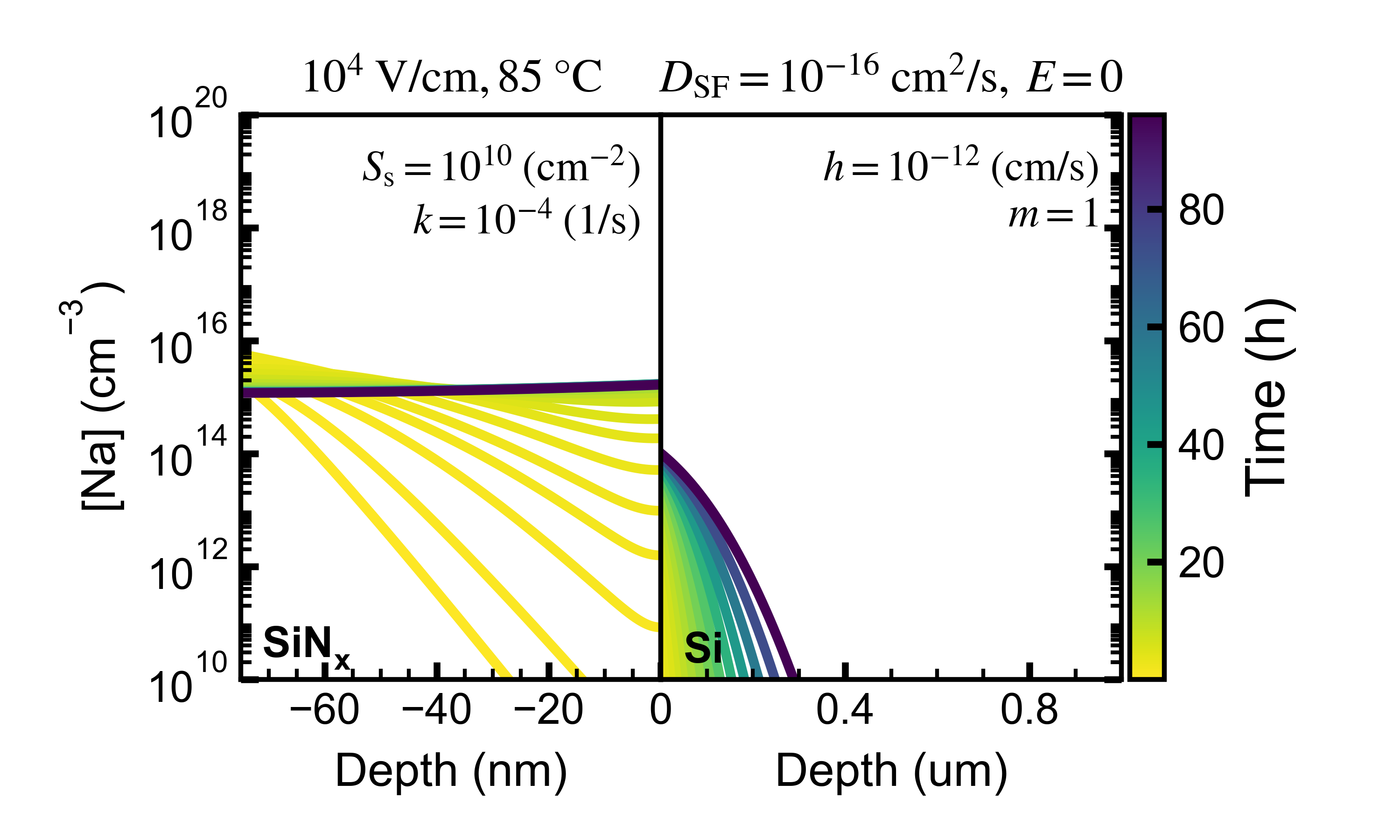
Example of a concentration plot from the batch analysis.
This is an example of a \(P_{\mathrm{mpp}}\) plot
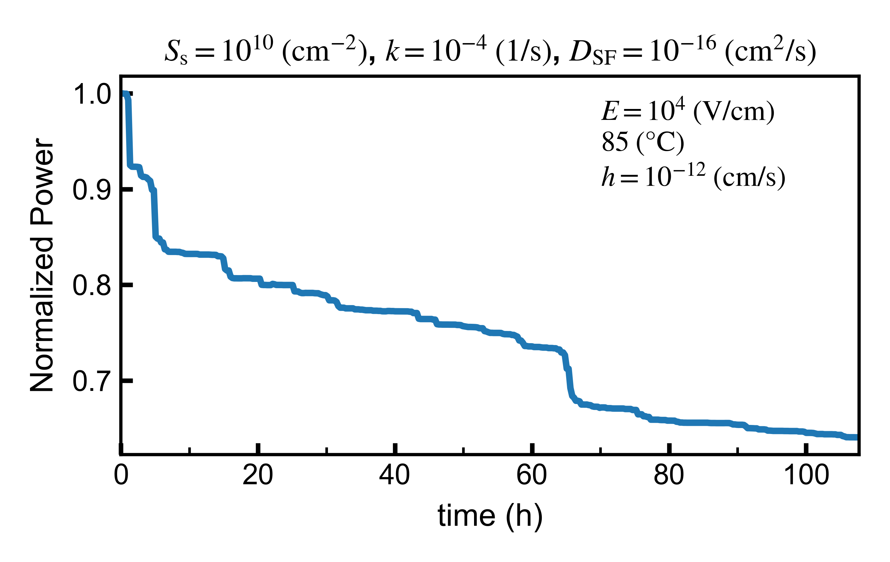
Example of a \(P_{\mathrm{mpp}}\) plot from the batch analysis.